| Oracle® OLAP Application Developer's Guide, 10g Release 2 (10.2.0.3) Part Number B14349-03 |
|
|
View PDF |
| Oracle® OLAP Application Developer's Guide, 10g Release 2 (10.2.0.3) Part Number B14349-03 |
|
|
View PDF |
An analytic workspace always returns summary data to a query as needed. While the analytic workspace may store data, for example, at the day level, it will return a result at the quarter or year level without requiring a calculation in the query. This chapter explains how to optimize the unique aggregation subsystem of Oracle OLAP to provide the best performance for both data maintenance and querying.
This chapter contains the following topics:
Aggregation is the process of consolidating multiple values into a single value. For example, data can be collected on a daily basis and aggregated into a value for the week, the weekly data can be aggregated into a value for the month, and so on. Aggregation allows patterns in the data to emerge, and these patterns are the basis for analysis and decision making. When you define a data model with hierarchical dimensions, you are providing the framework in which aggregate data can be calculated.
Aggregation is frequently called summarization, and aggregate data is called summary data. While the most frequently used aggregation operator is Sum, there are many other operators, such as Average, First, Last, Minimum, and Maximum. Oracle OLAP also supports weighted and hierarchical methods. Following are some simple diagrams showing how the basic types of operators work. For descriptions of all the operators, refer to "Aggregation Operators".
Figure 7-1 shows a simple hierarchy with four children and one parent value. Three of the children have values, while the fourth is empty. This empty cell has a null or NA value. The Sum operator calculates a value of 12 (2 + 4 + 6) for the parent value.
Figure 7-1 Summary Aggregation in a Simple Hierarchy

The Average operator calculates the average of all real data, producing an aggregate value of 4 ((2 + 4 + 6)/3), as shown in Figure 7-2.
Figure 7-2 Average Aggregation in a Simple Hierarchy
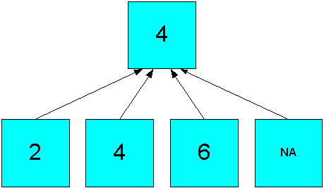
The hierarchical operators include null values in the count of cells. In Figure 7-3, the Hierarchical Average operator produces an aggregate value of 3 ((2 + 4 + 6 +NA)/4).
Figure 7-3 Hierarchical Average Aggregation in a Simple Hierarchy

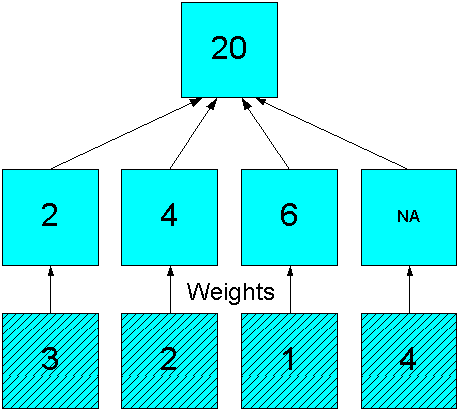
The weighted operators use the values in another measure to generate weighted values before performing the aggregation. Figure 7-4 shows how the simple sum of Figure 7-1 is altered by using weights ((3*2) + (2*4) + (1*6) +(4*NA)).
Figure 7-4 Weighted Sum Aggregation in a Simple Hierarchy
The creation and maintenance of summary data is a serious issue for DBAs. If no summary data is stored, then all summarizations must be performed in response to individual queries. This may slow the response time. At the other extreme, if all summary data is stored, then the database multiplies in size.
Relational schemas store aggregate data in materialized views and summary tables. The query rewrite feature of Oracle Database redirects queries for summary data from the fact tables to the materialized views. When predefined reports are run on a routine basis, the DBA knows which areas of the data are queried and what summary data is needed. This situation may be handled easily with a relatively small number of materialized views.
However, extensive use of ad-hoc queries and user-defined calculated measures create a random situation in which any part of the data store may be queried and summarized. Because a materialized view only has data for one combination of levels for the dimensions of the data, thousands of materialized views might be needed to provide coverage for most queries. A large number of materialized views requires extensive storage space and slows the query rewrite process for every request. When a particular materialized view is not available, the summary data is generated at runtime from the data in the fact table.
Analytic workspaces use an entirely different paradigm for managing aggregate data than relational tables. This paradigm is based on the dimensional model, which is inherent in analytic workspaces.
A cube is defined by its dimensions. Each cell in the cube is identified by a unique combination of dimension members, with one member from each dimension. The dimension members function as an index into the cube.
For each measure in the cube, a cell either has a data value or an NA value. While an NA is equivalent to empty or null, it is handled as the value of the cell. Thus, a cell with a value of NA can be queried the same as a cell with an actual data value. This is an important feature of dimensional data analysis, because it enables analysts to investigate the absence of data (that is, no activity) as well as the actual data.
A dimension is a list of all its members from the base to the most aggregate. Thus, a measure stores all of its data, regardless of its level of aggregation. There are no additional objects for storing aggregate data, and thus no need to redirect queries.
In an analytic workspace, a data load typically fetches data only at the lowest, or base, level. The data cells at the higher levels are empty until the values are calculated from the base values.
Table 7-1 shows a small portion of the Global Sales measure before aggregation.
The Channel dimension is set to a single base-level member named Catalog.
The Product dimension is set to a single base-level member named Sentinel Financial.
The Time dimension is set to Jul-04 and its ancestors, Q3-04 and 2004.
The Customer dimension is set to KOSH Enterprises Boston and its ancestors, United States, North America, and All Customers.
Out of the 12 cells shown, only one has a data value. If the three ancestors of Sentinel Financial and the one ancestor of Catalog were added, then this number would expand to one out of 96 cells.
Table 7-1 Portion of Sales Data Before Aggregation
| CatalogSentinel Financial | 2004 | Q3-04 | Jul-04 |
|---|---|---|---|
|
All Customers |
|
|
|
|
North America |
|
|
|
|
United States |
|
|
|
|
KOSH Entrpr Boston |
|
|
|
Nonetheless, the data is always presented to the application as fully solved; that is, both detail and summary values are provided, without requiring that calculations be specified in the query.
In an analytic workspace, aggregate data is generated at two distinct times:
As part of the build procedure. You can calculate and store all of the aggregates, none, or a portion of them. Calculated values are stored in the analytic workspace and shared by all sessions. This is often called pre-aggregation.
In response to a query. Any "missing" aggregate data will be calculated for the query, even if the analytic workspace has no stored aggregate data. Calculated values may be cached for use throughout a session, but they are not shared among sessions. This is often called aggregating on the fly.
If your dimensions have multiple hierarchies or if the hierarchies have many levels, then fully aggregating the measures can increase the size of your analytic workspace (and thus your database) geometrically. At the same time, much of the intermediate level data may be accessed infrequently or not at all.
The most effective method of summarizing data in any analytic workspace is by storing some aggregates and calculating others on the fly. When choosing which aggregate values to store, your goal is to select those that require time- and resource-intensive calculations. Calculations that can be performed quickly can be left until runtime.
Table 7-2 shows the same portion of the Global Sales measure after it has been aggregated as part of the data maintenance process. The Warehouse level of Customer and the Year level of time have been calculated and stored. Out of the 12 cells shown, four now have data values, which is one-third the total. The entire measure has this ratio when Channel and Product are fully aggregated during maintenance.
Table 7-2 Portion of Sales Data After Data Maintenance Aggregation
| CatalogSentinel Financial | 2004 | Q3-04 | Jul-04 |
|---|---|---|---|
|
All Customers |
|
|
|
|
North America |
|
|
|
|
United States |
|
|
|
|
KOSH Entrpr Boston |
|
|
|
When an application queries the analytic workspace, either the aggregate values have already been calculated and can simply be retrieved, or they can be calculated on the fly from a small number of stored aggregates. In addition, you can choose to cache aggregate values for the duration of a session, so that they are calculated on the fly only once. Table 7-3 shows the Sales measure when it is fully aggregated in response to a query. Eight values are calculated on the fly to return the answer set to the client.
Table 7-3 Portion of Sales Data Fully Aggregated For a Query
| CatalogSentinel Financial | 2004 | Q3-04 | Jul-04 |
|---|---|---|---|
|
All Customers |
|
|
|
|
North America |
|
|
|
|
United States |
|
|
|
|
KOSH Entrpr Boston |
|
|
|
The strategy for aggregation shown in "Basic Strategies for Aggregating Data" is called skip-level aggregation, because some levels are stored and others are skipped until runtime. The success of this strategy depends on choosing the right levels to skip, which are those that can be calculated quickly in response to a query.
Note:
Skip-level aggregation is used only for regular (non-compressed) composites. For the recommended strategy for compressed composites, refer to "Aggregating Compressed Composites".As a general rule, you should skip levels for only one or two dimensions and for no more than half of the dimensions of the cube. Choose the dimensions with the most levels in their hierarchies for skip-level aggregation.
Slower varying dimensions take longer to aggregate because the data is scattered throughout its storage space. If you are optimizing for data maintenance, then fully aggregate the faster varying dimensions and use skip-level aggregation on the slower varying dimensions.
You can identify the best levels to skip by determining the ratio of dimension members at each level, and keeping the ratio of members to be rolled up on the fly at approximately 10:1 or less. This ratio assures that all answer sets can be returned quickly. Either a data value is stored in the analytic workspace so it can simply be retrieved, or it can be calculated quickly from 10 stored values.
This 10:1 rule is best applied with some judgment. You might want to permit a higher ratio for levels that you know are seldom accessed. Or you might want to store levels at a lower ratio if you know they have heavy use. Generally, you should strive for a lower ratio instead of a higher one to maintain the best performance.
Aggregation rules identify how and when the aggregate values are calculated. You define the aggregation rules for each cube, and you can override these rules by defining new ones for a particular measure.
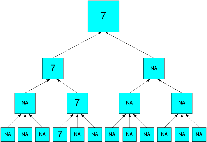
Compressed composites are used to store extremely sparse data. They are designed specifically to handle data structures in which several levels may store the same value. Figure 7-5 shows an aggregation in which one out of 12 cells has a data value. The skip-level strategy described in "Aggregating Non-Compressed Composites" does not produce any benefit under these circumstances.
Figure 7-5 Aggregation of Very Sparse Data
Use this aggregation strategy for compressed cubes:
Identify the dimension with the most members. If several dimensions have about the same number, then choose the dimension with the most levels. Do not pre-aggregate this dimension.
Pre-aggregate all other dimensions up to, but not including, the top level, unless the next level down has a large number of members.
You can adjust these basic guidelines to the particular characteristics of your data. For example, you may skip levels that are seldom queried from pre-aggregation. Or you may need to pre-aggregate a level with a large number of child values, to provide acceptable run-time performance.
The previous guidelines provide an approach to aggregation that should help you meet these basic goals:
If you anticipate problems with one or more of these goals, then you should keep them in mind while devising your aggregation rules. Otherwise, you may need to make adjustments after the initial build, if you experience problems meeting all of these goals.
Often the problem can be solved by changing factors other than the aggregation rules, as described in the following topics.
Note:
Be sure to run the Sparsity Advisor so that the data is structured in the most efficient way. Refer to "Using the Sparsity Advisor".Most organizations allocate a batch window in which all data maintenance must be complete. If you are unable to finish refreshing the data in the allotted time, then you can make the following adjustments.
The more levels that you aggregate for storage, the longer the maintenance process will take. Review your reasons for choosing levels for pre-aggregation. If you know that some levels are seldom queried, you may skip them during the builds. Exercise care in skipping additional levels, however, because you run the risk of degrading run-time performance.
Be sure that you have set the database initialization parameters correctly for data maintenance, as described in "Initialization Parameters for Oracle OLAP". You can make significant improvements in build performance by setting SGA_TARGET, PGA_AGGREGATE_TARGET, and JOB_QUEUE_PROCESSES.
After the initial build, you can save time by aggregating only newly loaded values, instead of aggregating all of them again. Partial aggregation is a choice you can make in the Maintenance Wizard.
Analytic workspaces are stored in partitioned tables, and you can create partitioned cubes. You can use these partitions to stripe the data across several disks, thus avoiding bottlenecks in I/O operations, if you have purchased the partitioning option to Oracle Database.
See Also:
Chapter 6, "Administering Oracle OLAP"Your analytic workspace must fit within the allocated resources. The more levels of aggregate data that you store, the larger the tablespaces must be to store the analytic workspace.
The data type is an important consideration when estimating the size of an analytic workspace. The most commonly used data types for measures are NUMBER and DECIMAL. The difference in size is significant: an unscaled NUMBER value is 22 bytes and a DECIMAL value is 8 bytes.
Refer to "Choosing a Data Type" for a comparison between these two data types.
An analytic workspace must provide good performance for end users. When pre-aggregation is done correctly, the response time for queries does not noticeably slow down. Analytic workspaces are optimized for multidimensional calculations, so that run-time summarizations should be extremely fast. However, runtime performance will suffer if the wrong choices were made.
If response time is poor, then review the decisions you made in skipping levels and find those that should be pre-aggregated. Try to identify and pre-aggregate those areas of the data that are queried heavily. Check the level on which you partitioned the cube. Remember that all levels above the partition are calculated on the fly. When partitioning over Time, the Month level is a much better choice than Day.
Read the recommendations given in the previous topics. The savings in maintenance time and disk storage may be used to pre-aggregate more of the data.
The aggregation rules defined for a cube or a measure are always performed over all dimension members. You can perform a partial aggregation only in a calculation plan and only for regular composites.
Note:
Do not set status for a compressed cube. All members must be in status.To aggregate over a portion of a measure, you select the dimension members that identify the cells containing the source data, using the Status page of the Aggregation property sheet. You do not need to select the target cells. All of the cells identified by the ancestors of the selected dimension members are aggregated, either when you execute the calculation plan or when a user queries the measure.
When you select the dimension members, they are in status. This means that the dimension members have been selected for use in a calculation, a query, or other data manipulation. Likewise, out of status means that the dimension members have been excluded from use.
Figure 7-6 shows an aggregation in which the 12 months of 2006 are in status. Neither the quarters nor the year are in status, but aggregates are generated for all levels.
Figure 7-6 Sum Aggregation With All Source Values in Status
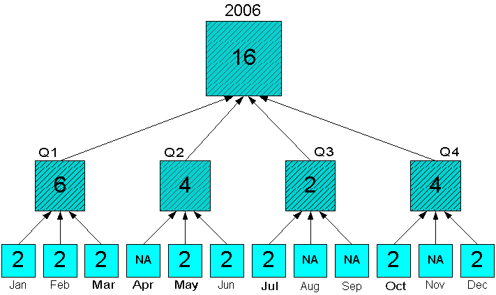
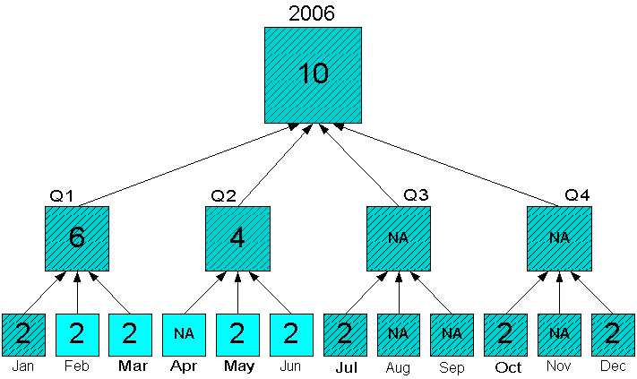
Figure 7-7 shows the same portion of data, but with only Feb to Jun in status. Aggregates are calculated only for Q1, Q2, and 2006. Note that Jan is included in the aggregation, even though it is out of status. The aggregation engine adds the ancestors, then the children to status before aggregating the data, as a means of maintaining the integrity of the data. The values for Jul to Dec are not included in the aggregation.
Figure 7-7 Sum Aggregation With Some Source Values Out of Status
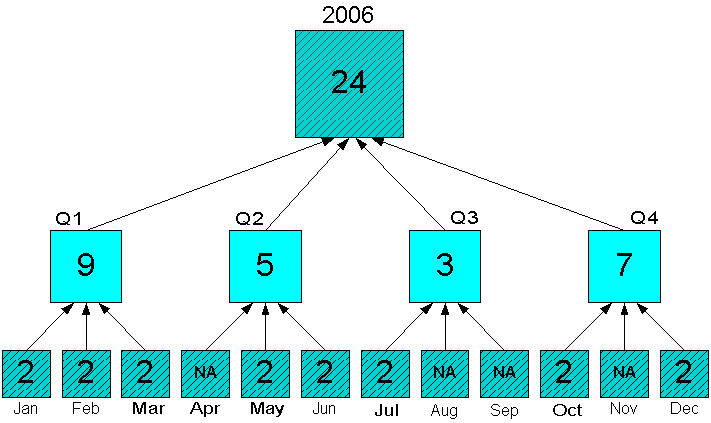
You may need to aggregate data that is stored in the middle of a hierarchy, perhaps if the data for a particular measure is not available or needed at the base level. You must be sure that the cells with the data are the lowest levels in the hierarchy in status. Figure 7-8 shows quarterly forecast data in status and aggregated to the year. The monthly values are not in status, and thus are excluded from the aggregation.
Figure 7-8 Sum Aggregation From the Quarterly Level
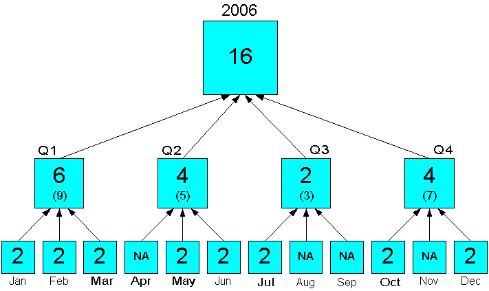
Aggregation begins at the lowest level in status and rolls up the hierarchy. The aggregate values will overwrite any pre-existing values higher in the hierarchy. Figure 7-9 shows that when the Month level is in status, those values will overwrite the forecast values at the Quarter level. The status of Quarter and Year has no effect on the aggregation.
Figure 7-9 Sum Aggregation From the Month Level Overwrites Quarters
Analytic Workspace Manager enables you to define aggregations at three different times. You can use whatever combination best suits your needs:
Cube. You can define default aggregation rules for all measures in a cube by defining them just once. You define these rules when creating or modifying a cube.
Measure. You can define unique aggregation rules for a particular measure that will override the default cube rules. You define these rules when creating or modifying a measure. You cannot specify aggregation rules for individual measures for compressed cubes.
Calculation Plan. You can define rules for one or more measures and determine the order in which the measures are calculated. In this way, you can support dependencies among the measures and the calculations, such as aggregating data that is generated by a forecast. You define these rules when creating or modifying a calculation plan. This type of aggregation is performed after the measures are aggregated using either the Cube or the Measure rules.
Note:
All measures are aggregated during data maintenance using the rules defined for the cube or the rules defined for the measure. Any additional aggregation rules defined in a calculation plan are calculated separately.Regardless of the level at which you define the summarization rules, the basic decisions and the user interface are the same:
Select an aggregation operator and, depending on the operator, a weight measure on the Rules tab.
Select the levels for storing values on the Summarize To tab.
To aggregate a measure using the cube rules:
On the General page of the Cube property sheet, select Use Default Aggregation Plan for Cube Aggregation.
On the General page of the Measure property sheet, select Use Aggregation Specification From the Cube.
To aggregate a measure using its individual rules:
On the General page of the Cube property sheet, select Use Default Aggregation Plan for Cube Aggregation.
Any measure in the cube without its own individual rules will use this default plan.
On the General page of the Measure property sheet, select Override the Aggregation Specification of the Cube.
To aggregate a measure using a calculation plan:
Define the aggregation rules for the measure or the cube, as described previously.
You can aggregate all the values first, then execute the calculation plan to overwrite a portion of the aggregate values. Or you can define the rules for the measure so that no aggregates are created during data maintenance.
Create a calculation plan that will aggregate all or part of the measure.
To aggregate all measures in a cube using a calculation plan:
On the General page of the Cube property sheet, clear the Use Default Aggregation Plan for Cube Aggregation box.
Create a calculation plan containing one or more aggregation steps that will aggregate all measures in the cube.
Analytic workspaces provide an extensive list of aggregation methods, including weighted, hierarchical, and weighted hierarchical methods.
These are the basic aggregation operators:
Average: Adds non-null data values, then divides the sum by the number of data values that were added together.
First Non-NA Data Value: The first real data value.
Last Non-NA Data Value: The last real data value.
Maximum: The largest data value among the children of each parent.
Minimum: The smallest data value among the children of each parent.
Nonadditive: Do not aggregate any data for this dimension.
Sum: Adds data values.
These are the hierarchical operators. They include all cells identified by the hierarchy in the calculations, whether or not the cells contain data. You should use these operators only when you want null values to be treated as zeroes instead of as missing data.
Hierarchical Average: Adds data values, then divides the sum by the number of the children in the dimension hierarchy. Unlike Average, which counts only non-null children, hierarchical average counts all of the logical children of a parent, regardless of whether each child does or does not have a value.
Hierarchical First Member: The first data value in the hierarchy, even when that value is null.
Hierarchical Last Member: The last data value in the hierarchy, even when that value is null.
Hierarchical Weighted Average: Multiplies non-null child data values by their corresponding weight values, then divides the result by the sum of the weight values. Unlike Weighted Average, Hierarchical Weighted Average includes weight values in the denominator sum even when the corresponding child values are null.
Hierarchical Weighted First: The first data value in the hierarchy multiplied by its corresponding weight value, even when that value is null.
Hierarchical Weighted Last: The last data value in the hierarchy multiplied by its corresponding weight value, even when that value is null.
These are the scaled and weighted aggregation operators. They require a measure containing the weights in the same cube.
Scaled Sum: Adds the value of a weight object to each data value, then adds the data values.
Weighted Average: Multiplies each data value by a weight factor, adds the data values, and then divides that result by the sum of the weight factors.
Weighted First: The first non-null data value multiplied by its corresponding weight value.
Weighted Last: The last non-null data value multiplied by its corresponding weight value.
Weighted Sum: Multiplies each data value by a weight factor, then adds the data values.
The Global data set is a good candidate for skip-level aggregation. This example discusses aggregation of the Units Cube, which has four dimensions: Time, Customer, Product, and Channel. You could skip levels on one or two dimensions. For this example, skip levels on only one dimension; because Global is small, precalculating the additional levels does not create a problem with time or disk space.
The Customer dimension has two hierarchies with a total of seven levels. Because it has the most levels of any dimension, it is the best choice for skipping levels.
To identify the levels to be precalculated, you must know the number of dimension members at each level. You can easily acquire this information in SQL, using this SQL command:
SELECT COUNT(DISTINCT ship_to_id), COUNT(DISTINCT warehouse_id),
COUNT(DISTINCT region_id),COUNT(DISTINCT total_customer_id),
COUNT(DISTINCT account_id), COUNT(DISTINCT market_segment_id),
COUNT(DISTINCT total_market_id), FROM global.customer_dim;
Global is a very small data set, so few adjacent levels have the desired 10:1 ratio of children-to-parent dimension members. Table 7-4 and Table 7-5 identify the appropriate levels to be calculated and stored for the two hierarchies. Only eight members are stored out of a total of 45 aggregate members.
On the Summarize To page for the Units Cube, select the precalculated levels for Customer, and select all levels for Time, Product, and Channel.
Table 7-4 Precalculated Levels in the Customer Shipments Hierarchy
| Level | Members | Precalculate? |
|---|---|---|
|
|
1 |
No |
|
|
3 |
Yes |
|
|
11 |
No |
|
|
61 |
Yes |
Table 7-5 Precalculated Levels in the Customer Market Segment Hierarchy
| Level | Members | Precalculate? |
|---|---|---|
|
|
1 |
No |
|
|
5 |
Yes |
|
|
24 |
No |
|
|
61 |
Yes |
Figure 7-10 shows this selection on the Summarize To page of the Units Cube property sheet.
Sales History is a very sparse data set, so it uses compressed composites for all cubes. You should fully aggregate all but the largest dimension. Table 7-6 shows the number of base-level members for each dimension. This information is easily acquired by counting the unique values in the dimension tables like this:
SELECT COUNT(DISTINCT time_id) FROM sh.times;
Because Customers is far larger than any of the other dimensions, you do not need to count the aggregate members or the number of levels to identify it as the largest one. On the Summarize To page for the cubes, deselect all levels for Customers and select all but the top level for Channels, Products, Promotions, and Times.